Ranking data helps you better understand key elements. Fortunately, Google Sheets’ RANK function makes it simple to rank data sets. Follow this post to find out how it works.
What’s RANK Function?
The RANK functions return a rank from a data set based on a given value in the data set. Find out where a student ranked on a test, for example. RANK could accomplish this by matching the student’s name to the test results. Google Sheets has three functions that enable you to rank data. Among them are the RANK function, RANK.EQ, and RANK.AVG. Although all functions behave identically, little tweaks may make them beneficial for certain applications.
Except when there are duplicate values in the data set, the RANK.EQ and RANK functions are similar and return the rank for the same values. The distinction between these two is that RANK is an older Excel function that may or may not be compatible with future versions. So, if you often go between Excel and Google Sheets, RANK.EQ is the way to go. However, it is recommended to migrate to Google Sheets finally. RANK.AVG is unique in that it delivers the average position of a dataset rather than counting duplicate values individually. Use this if you know your data contains unwanted duplicates that you cannot eliminate.
RANK Function Syntax
The RANK function in Google Sheets has three parameters, two of which are required to operate correctly and one of which is optional.
The syntax for the RANK function in Sheets is as follows.
=RANK(val, dataset, ascending)This formula’s parameters are as follows.
val – The value in the dataset you wish to calculate the rank. If the dataset does not have a numeric value in the required cells, the formula will return a #N/A error since the data is incorrect.
dataset – The array or cell range containing the data to be evaluated.
ascending – An optional parameter that specifies whether the values in the provided dataset are ordered ascending or descending. If the parameter is set to 0 (False), the greatest value in the dataset will be assigned a rank of 1. If this parameter is set to 1, the data’s lowest value will be ranked as 1.
The default value is FALSE or 0 if the third parameter is missing.
The parameters for RANK.EQ and RANK.AVG is the same as for the RANK formula. Nonetheless, here’s the syntax for each of them.
=RANK.EQ(val, dataset, ascending)=RANK.AVG(val, dataset, ascending)How To Use RANK Function In Google Sheets?
Now that we’ve covered the syntax and how it works, let’s look at how you can use this formula in your spreadsheets.
Using RANK Function
Nine students’ names and marks are included in the dataset below. We want to add a new column that displays a student’s rank depending on their score. Here are the steps you take to do this.
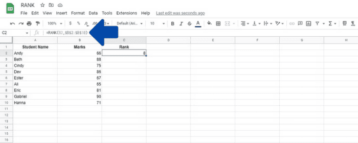
- To input a formula, click the cell where it is located. In our example, C2.
- To begin the formula, type Enter and the Equal (=) symbol.
- Enter the first half of the formula, RANK(.
- We want to enter the cell to rank as the first parameter. We seek Andy’s rank in this example; therefore, we choose cell B2, which has his marks.
- To separate the parameters, use a comma.
- The dataset parameter, which will be the cell range to search, must now be included. It is the cell range B2:B10 in this situation.
Note: To use the recommended autofill function to add the ranks to all the cells (Step 8), write this as $B$2:$B$10, which causes the formula to use absolute values.
- Add a closing bracket “)” to finish the formula and click Enter.
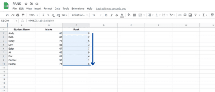
- Optional: Select the formula-containing cell. This will result in a blue border around that cell. Now, click and drag the thick blue dot in the lower-right corner downwards.
Using RANK.EQ Function
The RANK.EQ method returns the dataset’s rank, and if multiple instances of the same value are in the spreadsheet, the highest rank for the entries is returned. This function is the same as the RANK function. The following example shows this.
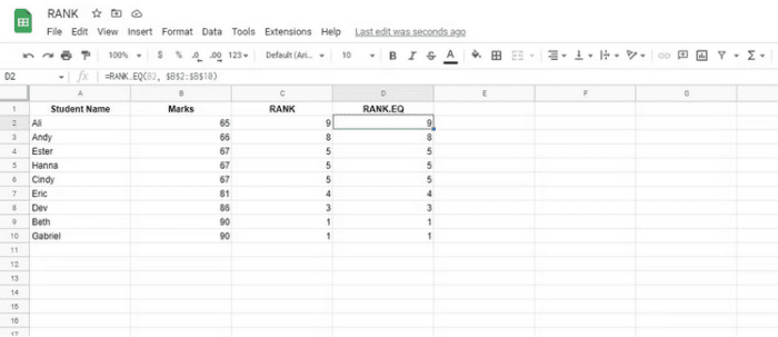
The spreadsheet has many occurrences of the same value in this example. As can be seen, both functions provide the same output, which means they may be substituted for each other in most circumstances.
Using RANK.AVG Function
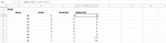
The RANK.AVG formula is a version of the RANK formula, which means its use is extremely similar, and you can apply it to your spreadsheet using the same steps we discussed before. However, the formula’s output is somewhat different. In this example, we used the RANK.AVG function on the same figures as previously.
The following are the instructions for using the RANK.AVG formula in your spreadsheet.
- Type the first portion of the formula, which is =RANK.AVG(, into the cell where you want to input the formula.
- For the first parameter, we want to enter the cell to rank. It is cell B2 in this scenario.
- Add a comma to separate the parameters and then write the second parameter, the cell range. It is the cell range $B$2:$B$10 in this example.
- To finish the formula, add a closing bracket “)”.
When you apply the function, the results will be similar to the RANK function. When the same value appears in many cells, the function will take the average rather than applying the same rank to all of them. For example, instead of 90 being the number one rank, it results in 1.5 since it averages rank 1 and 2 because there are two scores of 90. The score of 67 is presented as 6 since it is the average of 5, 6, and 7. This is in contrast to RANK.EQ, which gives the lowest possible rank to matched scores (5 in the example).
Using RANK Function With Arrays
We previously examined an example of using the RANK function in an existing dataset. This function, however, may also be used inside a single-cell array. This is a straightforward process.
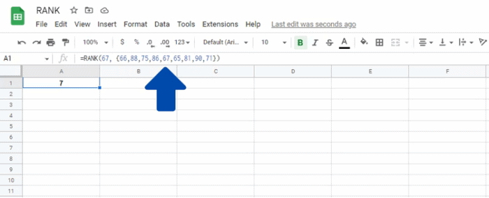
In the first parameter, write the number whose rank you want to find. We will write the numbers in the array for the second one. Here is the formula we used in this specific example.
=RANK(67, {66,88,75,86,67,65,81,90,71})As seen in the example, the cell displays where 67 ranks in the data set in the same manner as if the data were collected through cell references rather than being written directly into the formula.
Conclusion:
Google Sheets’ RANK functions are borderline intermediate. If you need help with them, review the guide again and create your spreadsheet to track each step. Google Sheets is a useful talent, and like with any new ability; it might take some time to master. But if you stick with it, you’ll be a pro in no time.